General method
For the encoding pipeline, a pretty much standard approach is used for either lossless (up to 12 bit grayscale) or quantized (lossy) encoding.
Both lossy and lossfree pipelines use a high speed huffman encoder with different code books and up to four contexts.
In the lossy mode, the image is decomposed into AC and DC subbands using a standard DWT approach. However, a predictor (called ‘sliding T’), different from JPEG2000 or JPEG LS is used and the special treatment is done by a particular bit plane shuffling. This makes the encoding logic much easier and allows to optimize the huffman tables in some cases ‘on the fly’.
Lossless mode
In lossless compression mode, it has turned out that the AC/DC subband decomposition does not beat the ‘Sliding T’ predictor in most cases. This observation comes close to statistics done on Lossless JPEG (not JPEG LS). The Sliding T Predictor (so forth STP) is context sensitive and is aware of up to 27 contexts, however in many cases only eight (‘STP8’) are used.
Example
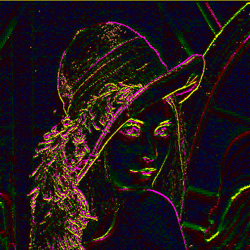
Here’s a visualization of the prediction step: The prediction image, generated via a lookup table, depicts the deviations from the differential coding using the STP8.
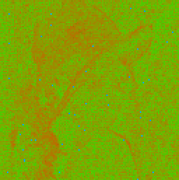
How well the compression performs, is seen in the so called ‘penalty map’. A very good compression (low entropy) can occur in the green areas, the more heading towards red, the more bits in the variable bit encoding are needed.

Lossy mode
In lossy mode, a quantization steps occurs inside the predictor loop (to eliminate errors) as well as a small optional quantization on the source data.
This introduces artefacts and may create quantization noise known from classical DPCM methods, although the predictor is not considered linear, but dependent from its pixel processing history (which is stored in a back log). The critical thing is to make sure the back log on encoder and decoder is the same.
This quantization step can occur both on AC and DC subbands, however for optimum compression, the 27 state ‘STP27’ was introduced to take care of special characteristics found in the AC subbands (‘HL’, ‘LH’, ‘HH’).
The interesting thing in the image below is that the artefacts at level 1 decomposition introduce too much entropy when using STP8 on the HH image. Very likely these are artefacts from repeated re-coding of the famous Lena image (although an assumed lossless PNG source was used).
The level 2 subband images depict how a quantized prediction reduces entropy such that a signification compression gain is achieved.
However, the STM8 lossless predictor performs better in this case than a lossless (reversible) DC/AC re-composition.


Wrap up
Compared to JPEG2000 with way much higher complexity, this approach performs less efficient on many high quality images, however it comes pretty close on a number of test images. For a particular application where the source data is correlated (e.g. Bayer Pattern), the STP8 performs quite well in lossless mode and does not require a complex hardware pipeline.
Lossy mode however takes some more complexity and only performs well with increasing quantization on AC/DC subbands. Depending on the quantization mode, either memory for lookup tables or DSP units for multiplication are required in the hardware pipeline.
Open items:
- Detailed statistics (being collected)
- Bit rate control (truncation mode)
- 16 bit grayscale: Not yet implemented
- NHW codec compatibility: Introduce YCoCg, Predictor?