Here’s a short step by step intro to install and run netpp on Windows10 (it will work likewise on older Windows versions):
- Download Python 2.7 (32 bit) and install it. Make sure to install for all users, otherwise the netpp installer will not find the Python directory and complain.
- Download and run:
[sdm_download id=”1349″ fancy=”1″] - Run the example server via Start Menu->netpp->Run example server. A warning will appear and request you to unblock the service, possibly. Then, a small example netpp server is listening on your local machine.
- Start the IDLE environment via Start Menu->Python 2.x->IDLE. Read more in detail below…
If you did not download Python before installing netpp, the netpp installer will throw a warning, but still continue.
First steps

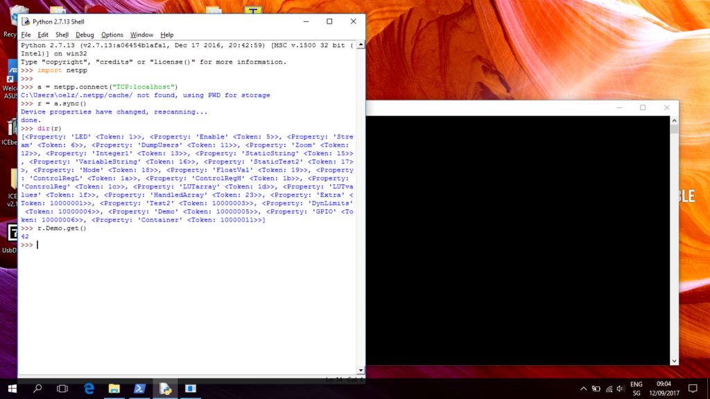
When you have started IDLE, first try to import the netpp module as shown in the screen shot. Then make a connection to your local example server using the .connect() method.
The .sync() command creates a local property tree with root node ‘r’. When first called, the device server is queried for all available properties, so this can take a long time on some systems. Once the query has completed, the tree is stored in a cache and is only reloaded, if the device properties have changed.
Note the message “using PWD for storage”. If you have no cache directory created, the cache will be installed in the current program’s working directory, which may not be desired. Create the folders ‘.netpp/cache’ in your home directory, then the warning will go away. If you ever need to manually delete the cache files, you will find them there.
Next, we are going to look at the properties. This is simply done the pythonish way using ‘dir’.
And last, we obtain a property value using the .get() method. Simple as that.
Using the Power shell
There are two command line utilities:
- master: Simple command line demo tool for netpp access
- netpp-cli: interactive netpp client
Open up a Power shell (or a legacy cmd.exe) and change directory to where your netpp binaries are installed, like
cd c:\Program Files (x86)\section5\netpp\bin
The master.exe is a very primitive command line tool for netpp device query. When run without arguments, it will display the available hubs and send out a broadcast on the local network for attached netpp devices. If your example server is running, you will see it listed. Try accessing it:
.\master TCP:192.168.56.1
and it will list the device’s properties.
The netpp-cli.exe is an interactive console with a bit more caching functionality and session character, i.e. when you made a connection, the device will reserve a session with you until you exit the CLI. This operation mode may be required on some more complex devices that work session based.
Make a connection to a device:
.\netpp-cli TCP:192.168.56.1
At the netpp prompt, type ‘?’. Now you can just get a property value by typing its property name, like Container.Test. When you append a value, you can change a property, likewise.
Process viewer/browser support
To use the predefined GUI process control based on the free pvbrowser (see github repository), you need a demo setup based on a modhub or another Linux embedded demo setup running a pvhub server. This assumes a netpp node setup with default design.
- Start the pvbrowser on your PC
- Enter the URL
pv://modhub/netpp:UDP:192.168.0.5:2016
into the pvbrowser for a direct connection to the netpp node (assuming default IP at 192.168.0.5). Replace ‘modhub’ by the IP address of your pvhub server host.
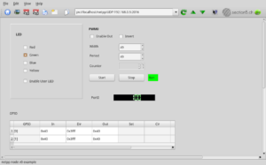
- The process viewer should display something like below:

Troubleshooting
There are some known issues with the evaluation release netpp 0.5-rc1 on Windows and IDLE:
- When a cache directory was not created ($HOME\.netpp\cache), Python(IDLE) will report:
C:\Users\me\/.netpp/cache not found, using PWD for storage
This is mostly not a problem, however when access rights are limited, creating the cache can fail. Create this directory in your $HOME then.
- Upon synchronization, a failure can occur when a cache created from an older netpp version is found:
r = a.sync()

...

IndexError: tuple index out of range
Search for the corresponding *.pyp file and remove it
Further resources:
LabVIEW wrapper based on OpenG LabPython
- LabVIEW project build (testing): [sdm_download id=”1444″ fancy=”0″]
Documentation:
- netpp HOWTO: [sdm_download id=”1350″ fancy=”0″]
- API reference OpenSource v0.3x [ HTML ]


