2017 – section5

Posted on 13. November 20179. November 2019 by m s

Setting up virtual CPU environment on Windows

This is a short howto to get a Linux specific Virtual Chip running on a Windows OS:

Download and install the Docker Toolbox
Download and install the Xming X-Server
Run ‘Docker Quickstart terminal’, normally installed on your desktop. Be patient, the environment takes some time to start up
Download MaSoCist docker container:
```
docker pull hackfin/masocist
```
Optional: (GTKwave support): Prepare the Xming server by running XLaunch and configuring as follows using the Wizard:
- Multiple Windows
- Start no client
- No access control selected (Warning, this could cause security issues, depending on your system config)

Start the container using the script below

docker run -ti --rm -u masocist -w /home/masocist -e DISPLAY=192.168.99.1:0 \
-v /tmp/.X11-unix:/tmp/.X11-unix hackfin/masocist bash

You might save this script to a file like run.sh and start it next time from the Docker Quickstart terminal:

. run.sh

Depending on the MaSoCist release you’ve got, there are different install methods:

Opensource github

See README.md for most up to date build notes. GTKwave is not installed by default. Run

sudo apt-get update gtkwave

to install it.

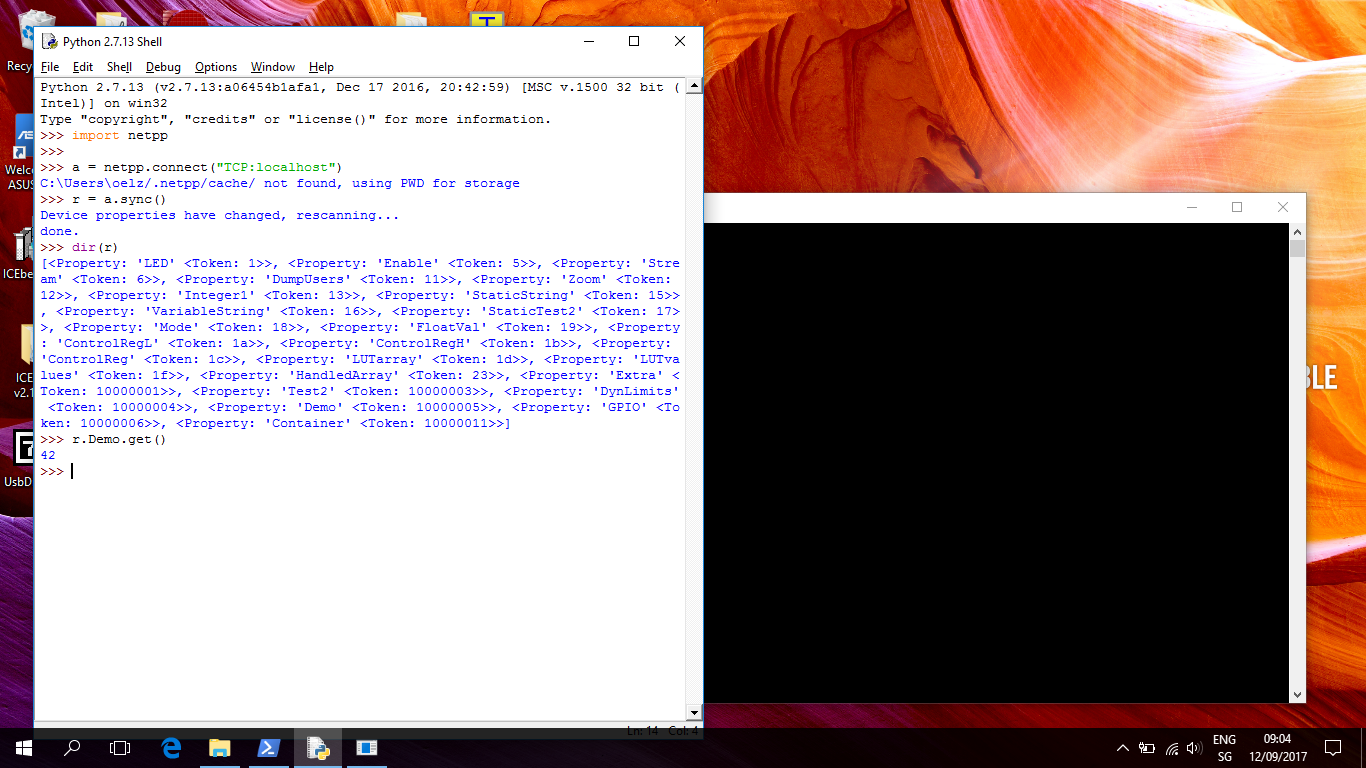
When you have X support enabled, you can, after building a virtual board, run

make -C sim run

from the MaSoCist directory to start the interactive wave display simulation. If the board uses the virtual UART, you can now also connect to /tmp/virtualcom using minicom.

Custom ‘vendor’ license

You should have received a vendor-<YOUR_ORGANIZATION>.pdf for detailed setup notes, see ‘Quick start’ section.

A few more notes

All changes you will make to this docker container are void on exit. If this is not desired, remove the ‘–rm’ option and use the ‘docker ps -a’ and ‘docker start -i <container_id>’ commands to reenter your container. Consult the Docker documentation for details.
Closing the GTKwave window will not stop the simulation!
Ctrl-C on the console stops the simulation, but does not close the wave window
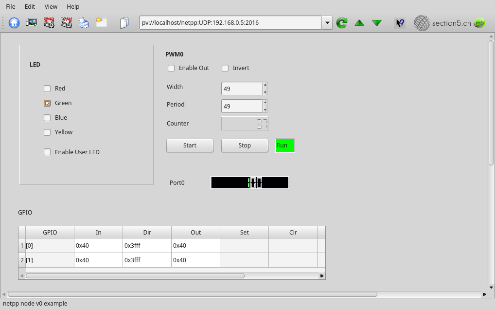
The UART output of the virtual SoC is printed on the console (“Hello!”). Virtual UART input is not supported on this system, but can be implemented using tools supporting virtual COM ports and Windows pipes.
Once you have the Docker container imported, you can alternatively use the Kitematic GUI and apply the above options, in particular:
- -v: Volume mounts to /tmp/.X11-unix
- -e: DISPLAY environment setting

Posted on 12. September 201722. March 2022 by M Strubel — 2 Comments

netpp for Windows quick start

Here’s a short step by step intro to install and run netpp on Windows10 (it will work likewise on older Windows versions):

Download Python 2.7 (32 bit) and install it. Make sure to install for all users, otherwise the netpp installer will not find the Python directory and complain.
Download and run:
[sdm_download id=”1349″ fancy=”1″]
Run the example server via Start Menu->netpp->Run example server. A warning will appear and request you to unblock the service, possibly. Then, a small example netpp server is listening on your local machine.
Start the IDLE environment via Start Menu->Python 2.x->IDLE. Read more in detail below…

If you did not download Python before installing netpp, the netpp installer will throw a warning, but still continue.

First steps

When you have started IDLE, first try to import the netpp module as shown in the screen shot. Then make a connection to your local example server using the .connect() method.

The .sync() command creates a local property tree with root node ‘r’. When first called, the device server is queried for all available properties, so this can take a long time on some systems. Once the query has completed, the tree is stored in a cache and is only reloaded, if the device properties have changed.

Note the message “using PWD for storage”. If you have no cache directory created, the cache will be installed in the current program’s working directory, which may not be desired. Create the folders ‘.netpp/cache’ in your home directory, then the warning will go away. If you ever need to manually delete the cache files, you will find them there.

Next, we are going to look at the properties. This is simply done the pythonish way using ‘dir’.

And last, we obtain a property value using the .get() method. Simple as that.

Using the Power shell

There are two command line utilities:

master: Simple command line demo tool for netpp access
netpp-cli: interactive netpp client

Open up a Power shell (or a legacy cmd.exe) and change directory to where your netpp binaries are installed, like

cd c:\Program Files (x86)\section5\netpp\bin

The master.exe is a very primitive command line tool for netpp device query. When run without arguments, it will display the available hubs and send out a broadcast on the local network for attached netpp devices. If your example server is running, you will see it listed. Try accessing it:

.\master TCP:192.168.56.1

and it will list the device’s properties.

The netpp-cli.exe is an interactive console with a bit more caching functionality and session character, i.e. when you made a connection, the device will reserve a session with you until you exit the CLI. This operation mode may be required on some more complex devices that work session based.

Make a connection to a device:

.\netpp-cli TCP:192.168.56.1

At the netpp prompt, type ‘?’. Now you can just get a property value by typing its property name, like Container.Test. When you append a value, you can change a property, likewise.

Process viewer/browser support

To use the predefined GUI process control based on the free pvbrowser (see github repository), you need a demo setup based on a modhub or another Linux embedded demo setup running a pvhub server. This assumes a netpp node setup with default design.

Start the pvbrowser on your PC
Enter the URL
```
pv://modhub/netpp:UDP:192.168.0.5:2016
```
into the pvbrowser for a direct connection to the netpp node (assuming default IP at 192.168.0.5). Replace ‘modhub’ by the IP address of your pvhub server host.
The process viewer should display something like below:

PVbrowser netpp node v0 — PVbrowser netpp node example

Troubleshooting

There are some known issues with the evaluation release netpp 0.5-rc1 on Windows and IDLE:

When a cache directory was not created ($HOME\.netpp\cache), Python(IDLE) will report:
```
C:\Users\me\/.netpp/cache not found, using PWD for storage
```
This is mostly not a problem, however when access rights are limited, creating the cache can fail. Create this directory in your $HOME then.
Upon synchronization, a failure can occur when a cache created from an older netpp version is found:
```
r = a.sync()

...

IndexError: tuple index out of range
```
Search for the corresponding *.pyp file and remove it

Further resources:

LabVIEW wrapper based on OpenG LabPython

LabVIEW project build (testing): [sdm_download id=”1444″ fancy=”0″]

Documentation:

netpp HOWTO: [sdm_download id=”1350″ fancy=”0″]
API reference OpenSource v0.3x [ HTML ]

Posted on 11. September 201719. January 2020 by m s — Leave a comment

Image compression prediction techniques

Prediction techniques are present in almost any approach to image compression, be it lossless or lossy. The general idea of a predictor is, to extrapolate a pixel from its neighbours, i.e. assuming it has a specific value. The difference between this assumed value and the effective value is regarded as error. For a round trip coding, i.e. forward and inverse transformation, it is only required to store a reference, prediction history and the errors.

Since these errors are – seen from a statistical distribution – rather limited, the encoding can happen effectively with less bits than the eight bits normally used per pixel channel.

A simple predictor

A very simple predictor tries to predict pixel values based on the previous scan line or pixel row. It evaluates the pixels [0, 1, 2] as shown below to extrapolate the value of [X]:

00  11  22 ...
##  XX  ##

Running this through a test image and storing only the error, we get something like below:

Test image from unsplash, scaled/cropped

The prediction error image was quantized to make the potential compression gain more visible.

By simple bit plane reshuffling and entropy coding techniques deployed by the JPEG XS format, our predictor experiment allows to compress the above image lossless by roughly factor two. Using Wavelet decomposition, lossless compression can be achieved up to factor four. By quantization (that will introduce information loss), much higher compression in the range of 1:10-1:20 can be achieved with quality compareable to the classic JPEG format, however with reduced block artefacts at higher compression.

Context sensitivity and adaptivity

When recompressing images, artefacts can arise that are hard to re-compress. Likewise, bayer pattern raw sensor images converted to YUV or RGB values can lead to frequency artefacts that cause higher entropy. Our approach uses a very simple, context sensitive predictor based on a 8-state finite state machine where the decision on what state is chosen next is based on a simple history and a comparison. The image below shows a typical error distribution for these eight states. For a normal grayscale image, the statistical distribution is alike for each state. For artefact-tainted images, the distribution can be rather distorted.

Refined context tracker

Experiments with a higher number of contexts and a complex tracking history yielded a better compression for artefact-tainted images – under certain circumstances. The above T shaped predictor (internally named ‘STP8’ for sliding T predictor) was enhanced to 27 states (‘STP27’) in particular to perform well in the following scenarios:

JPEG recompression artefacts
Bayer pattern artefacts (Bayer to YUV422)
Custom color pattern experiments (undocumented)

Each of these artefact scenarios requires a specific default parameter setting for the STP27. A classification of pixels is then done ‘on the fly’ and adaptive compression is applied. This showed a significant improvement over the STP8, but introduces some complexity of the hardware state machine and requires a rather large huffman coding table.

In simulation experiments with a number of ‘classic’ test images, this turned out to actually beat lossless wavelet compression.

Hardware implementation

Using our proprietary FLiX coprocessing engine, a hardware based pipeline can be generated that uses FPGA technology to compress grayscale images at a very high data rate (up to 200 Mpixel/s per channel). Basically, no multiplication is required for the ‘baseline’ variant. For images with higher amount of artefacts however, decorrelation approaches are deployed that will require multiplications, and a feedback regulation similar to convolutional neuronal networks. This is still under scrutiny. For most sensor imagery however, it appears that the compression gain is not excessive. Update: Obsolete with STP27 implementation.

Update: 2.4.2015
Repub: 11.9.2017 [Replace images]