Author: m s

Prediction techniques are present in almost any approach to image compression, be it lossless or lossy. The general idea of a predictor is, to extrapolate a pixel from its neighbours, i.e. assuming it has a specific value. The difference between this assumed value and the effective value is regarded as error. For a round trip coding, i.e. forward and inverse transformation, it is only required to store a reference, prediction history and the errors.

Since these errors are – seen from a statistical distribution – rather limited, the encoding can happen effectively with less bits than the eight bits normally used per pixel channel.

A simple predictor

A very simple predictor tries to predict pixel values based on the previous scan line or pixel row. It evaluates the pixels [0, 1, 2] as shown below to extrapolate the value of [X]:

00  11  22 ...
##  XX  ##

Running this through a test image and storing only the error, we get something like below:

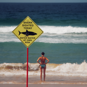
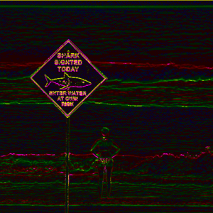
The prediction error image was quantized to make the potential compression gain more visible.

By simple bit plane reshuffling and entropy coding techniques deployed by the JPEG XS format, our predictor experiment allows to compress the above image lossless by roughly factor two. Using Wavelet decomposition, lossless compression can be achieved up to factor four. By quantization (that will introduce information loss), much higher compression in the range of 1:10-1:20 can be achieved with quality compareable to the classic JPEG format, however with reduced block artefacts at higher compression.

Context sensitivity and adaptivity

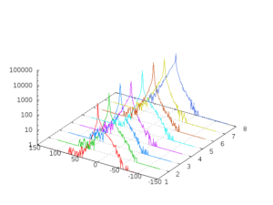
When recompressing images, artefacts can arise that are hard to re-compress. Likewise, bayer pattern raw sensor images converted to YUV or RGB values can lead to frequency artefacts that cause higher entropy.  Our approach uses a very simple, context sensitive predictor based on a 8-state finite state machine where the decision on what state is chosen next is based on a simple history and a comparison. The image below shows a typical error distribution for these eight states. For a normal grayscale image, the statistical distribution is alike for each state. For artefact-tainted images, the distribution can be rather distorted.

Refined context tracker

Experiments with a higher number of contexts and a complex tracking history yielded a better compression for artefact-tainted images – under certain circumstances. The above T shaped predictor (internally named ‘STP8’ for sliding T predictor) was enhanced to 27 states (‘STP27’) in particular to perform well in the following scenarios:

• JPEG recompression artefacts
• Bayer pattern artefacts (Bayer to YUV422)
• Custom color pattern experiments (undocumented)

Each of these artefact scenarios requires a specific default parameter setting for the STP27. A classification of pixels is then done ‘on the fly’ and adaptive compression is applied. This showed a significant improvement over the STP8, but introduces some complexity of the hardware state machine and requires a rather large huffman coding table.

In simulation experiments with a number of ‘classic’ test images, this turned out to actually beat lossless wavelet compression.

Hardware implementation

Using our proprietary FLiX coprocessing engine, a hardware based pipeline can be generated that uses FPGA technology to compress grayscale images at a very high data rate (up to 200 Mpixel/s per channel). Basically, no multiplication is required for the ‘baseline’ variant. For images with higher amount of artefacts however, decorrelation approaches are deployed that will require multiplications, and a feedback regulation similar to convolutional neuronal networks. This is still under scrutiny. For most sensor imagery however, it appears that the compression gain is not excessive. Update: Obsolete with STP27 implementation.

---

Update: 2.4.2015
Repub: 11.9.2017 [Replace images]