Posted on 2 Comments

In Circuit Emulation for MIPS soft CPU

Many developers got used to this: Plug in a JTAG connector to your embedded target and debug the misbehaviour down to the hardware. No longer a luxury, isn’t it?
When you move on to a soft core from opencores.org for a simple SoC solution on FPGA, it may be. Most of them don’t have a TAP – a Test Access Port – like other off the shelf ARM cores.

We had pimped a ZPU soft core with in circuit emulation features a while ago (In Circuit Emulation for the ZPU). This enabled us to connect to a hardware ZPU core with the GNU debugger like we would attach to for example a Blackfin, msp430, you name it.

Coming across various MIPS compatible IP cores without debug facilities, the urge came up to create a standard test access port that would work on this architecture as well. There is an existing Debug standard called EJTAG, but it turned out way more complex to implement than simple In Circuit Emulation (ICE) using the above TAP from the ZPU.

So we would like to do the same as with the ZPU:

  • Compile programs with the <arch>-elf-gcc
  • Download programs into the FPGA hardware using GDB
  • set breakpoints, inspect and manipulate values and registers, etc.
  • Run a little “chip scope”

Would that work without killer efforts?

Yes, it would. But we’re not releasing the white rabbit yet. Stay tuned for embedded world 2013 in Nuremberg in February. We (Rene Doß from Dossmatik GmbH Germany and myself) are going to show some interesting stuff that will boost your SoC development big time by using known architectures and debug tools.

His MIPS compatible Mais CPU is on the way to become stable, and turns out to be a quick bastard while being stingy on resources.

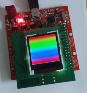
For a sneak peek, here’s some candy from the synthesizer (including I/O for the LCD as shown below):

Selected Device : 3s250evq100-5

Number of Slices:                     1172  out of   2448    47%
Number of Slice Flip Flops:            904  out of   4896    18%
Number of 4 input LUTs:               2230  out of   4896    45%
Number of IOs:                          15
Number of bonded IOBs:                  15  out of     66    22%
Number of BRAMs:                         2  out of     12    16%
Number of GCLKs:                         3  out of     24    12%

And for the timing:

Minimum period: 13.498ns (Maximum Frequency: 74.084MHz)
Mais on Papilio with TFT wing

Update: Here’s a link to the presentation (as PDF) given on the embedded world 2013 in Nuremberg:

presentation-2013

Posted on Leave a comment

Unlocking USB sticks from Ubuntu/Linux

Just recently, I bought a USB stick from a major discounter. When sticking it in, it showed some preinstalled software to configure a hidden partition. Ok, nice feature, when you lose your stick.

Let’s have a look at the outlines:

Bus 002 Device 035: ID 13fe:3623 Kingston Technology Company Inc.

It is branded as a Maxell pen drive.

I will not go into the security details, but take my advice and don’t assume your data is well encrypted or really secure. An electronics Pro will be able to read out your data!

Anyhow, so I have my hidden partition, but I’d like to see it from Linux, too (why would I use anything else, ha ha). Bummer, no Linux support. Not giving up early though. We know that a USB drive is in fact a SCSI disk, so it is all about sending the right vendor extension SCSI commands to the right target.

In Linux, this is simply done accessing a scsi generic device. Before losing any more words, here is the C source for it:

Kingston USB memory unlocker source code

You have to compile this utility yourself (do not ask for binaries, or you’ll be pushed with a soft cushion) and run it using sudo or as root (both potentially dangerous) and enter the correct password (when prompted with “Phrase:”) that you have entered when configuring the device under Windows. I’m afraid, no support for setting up the partitions and protection under Linux.

If the password is correct, the drive will reconnect automatically and show up in your file manager.

The Windows Lock tool will give you only a number of limited attempts trying to guess the password before the hidden partition is erased. It has not been tested whether this is a hardware feature or done by the software tool. Comments welcome.

Big fat WARNING: This is an experimental tool. Make sure you do *not* access your hard disk!

To determine the generic SCSI device, see the ‘dmesg’ output after sticking in the USB pen drive. My code above will do a check for the drive ID string, but this might not be paranoid enough.


Posted on 1 Comment

A full baseline pipelined JPEG encoder in VHDL

As described in a previous post, a framework was built to loop in a DCT hardware design into a software JPEG encoder for verification (and acceleration) purposes.

Turns out this strategy speeds up development a lot, and that the remaining modules on the way to a full hardware based and pipelined JPEG encoding solution weren’t a big job. Actually, I was expecting that this enhanced encoder would no longer fit into a small Spartan3E 250k. Wrong!

Have a look:

Device utilization summary:
---------------------------

Selected Device : 3s250evq100-5 

 Number of Slices:                     1567  out of   2448    64%  
 Number of Slice Flip Flops:           1063  out of   4896    21%  
 Number of 4 input LUTs:               2915  out of   4896    59%  
    Number used as logic:              2900
    Number used as Shift registers:      15
 Number of IOs:                          49
 Number of bonded IOBs:                  47  out of     66    71%  
 Number of BRAMs:                        12  out of     12   100%  
 Number of MULT18X18SIOs:                11  out of     12    91%  
 Number of GCLKs:                         2  out of     24     8%

JPEG encoder latency and timing

From the XST summary, we get:

Timing Summary:
---------------
Speed Grade: -5

   Minimum period: 13.449ns (Maximum Frequency: 74.353MHz)
   Minimum input arrival time before clock: 9.229ns
   Maximum output required time after clock: 6.532ns
   Maximum combinational path delay: 7.693ns

The timing is again optimistic, place and route normally deteriorates the latencies. The maximum clock is in fact the clock you can feed the JPEG encoder with pixel data (12 bit) without causing overflow. The output is a huffman coded byte stream that is typically embedded into a JFIF structure header, table data and the appropriate markers by a CPU.

There is quite some room for optimization, in fact, the best compromise of BRAM bandwidth and area has not yet been reached. Quite a few BRAMs ports are not used, but kept open to allow access through an external CPU, like for manipulation of the Huffman tables.

JPEG encoder waveforms

The last performance question might be the latency: how long does it take until encoded JPEG data appears after the first arriving pixel data? The above waveform snapshot should speak for itself: at 50MHz input clock, the latency is approx. 4 microseconds.

Colour encoding

We haven’t talked about colour yet. This is a complex subject, because there are many possibilities of encoding colour, but not really for the JPEG encoder. This is rather a matter of I/O sequencing and the proper colour conversion. As you might remember, a JPEG encoder does not encode three RGB channels, but in YUV space, which might be roughly described as: brightness, redness and blueness. The ‘greenness’ is implicitely included in this information. But why repeat what’s already nicely described: You find all the details right here on Wikipedia.

So, to encode all the colour, we just need properly separated data according to one of the interleaving schemes (4:2:0 or 4:2:2) and feed the MCU blocks of 8×8 pixels through the encoder while assserting the channel value (Y, Cb, Cr) on the channel_select input. Voilà.

Turns out that the Bayer Pattern that we receive from many optical colour sensors can be converted rather directly into YUV 4:2:0 space using the right setting four our Scatter-Gather unit (‘cottonpickens’ engine). With a tiny bit of software intervention through a soft core, we finally cover the entire colour processing stream. Proof below.

Colour JPEG
Colour JPEG output from the encoder
The original RGB photo

As you can see, the colours are quite not perfect yet compared with the original. This is a typical problem, that you get a greenish tint. We leave this to the colour optimization department 🙂

One more serious word: Just yesterday I’ve read the news and had to see that the person who changed the optical colour sensor industry, Bryce Bayer, has passed away. As a final “thank you” to his work, I’d like to post the Bayer Picture of the above.

Bayer pattern source image
Dedicated to Bryce Bayer